![Triggered_Event_as_Sum_Over_Histories. Observed Stochastic Motions
We are going to start this section proposing you to imagine what you’d see if you could magnify details as small as ~10-35 m. As an example, the hypotetical orbits where 113 years ago the British physicist Rutherford assumed the electron of the Hydrogen atom to be revolving around a nucleus. The effects of this permanent and randomly oriented oscillation of the electron are known since then. Effects hinted in the figure below: no orbit at all. It lies in this posterior observation one of the main reasons why Quantum Mechanics had to be created replacing the newtonian Mechanics. It was not an academic exercise: the progress of theories and their comparison with experimental and technological facts, around the end of the Nineteenth Century implied also a progressive divergence of what was considered causing what else. The motion of a particle, yet in the basic unidimensional case above on left side, is an example of this departure from the Classic concepts. The electron is affected by fluctuations of the electric field in vacuum, also named “ground state” or “zero-point” fluctuations, creating displacements with respect to the theoretical curve a true orbit should imply. Displacements nil on average, but huge when considering their root mean square. Then, the electric field truly felt by the electron is not the static one supposed around the (positive) proton. Zero-Point field random oscillations permeate all the space: they are not a feature of the matter, rather of the space itself. They are observed also freezing an ambient a few thousandths of kelvin degrees over the absolute zero, implying that their origin is non-thermal. To detect them and measure what the animation on side tries to show, are not necessary complex Laboratory equipments. In the following two examples. Example 1
Measurement of Electromagnetic Field Fluctuations. Imagine a common oscilloscope like the one here above:
Expose the 10.0 mm long metallic tip of its probe (an example in the figure below) to the electromagnetic field of a distant source, whose frequency is 1.0 MHz. Imagine a magnetic field B, measured where the oscilloscope’s probe emulates an antenna, amounting to 10-8 gauss.
For a spatial domain of this size, oscillating at that frequency, the fluctuation of the em field amounts to only ~10-17 gauss. Say, it is one hundred millions times smaller. Then definetely impossible to detect, lost in a sea of noise. Repeat the test after having cutted to < 1 mm the metallic exposed part of the probe:
now the quantum fluctuations dominate. An order of magnitude over the classically expected electromagnetic field, amounting to ~10-7 gauss. Reducing ten times the probe’s length, we reduced in the meantime the amount of mass-energy and space.
Conclusions:
The spatial domain, also when emptied by mass-energy (i.e., the probe's metallic tip) has its own electromagnetic field, and this results now ten times bigger than that induced by a power trasmitter. Space’s true nature starts to show itself.
Example 2
Measurement of Geometric Fluctuations
We frequently named concepts like: curvature of the geometry, curvature of the space, 3-dimensional geometry or 4-dimensional spacetime. These terms are frequently underestimated in their yield. On the opposite, after 1915, they refer to quantitatively defined amounts. Amounts whoever feels (the gravity) and can easily measure with small field devices named gravimeters. Gravimeters are equipments commonly used to measure variations in the Earth’s gravitational field. This last, a synonimous of the tidal effects due to the curvature and other peculiarities of the geometry of the space at the surface of the Earth. The field is not static, but varies continuously with time because of the movement of the masses.
The masses being primary sources of gravity variation are:
tides,
hydrology,
land uplift/subsidence,
ocean tide loading,
atmospheric loading;
changes in the Earth’s polar ice caps;
Sun;
Moon;
planets.
A number of different mechanical and optical schemes exist to measure this deflection, which in general is very small. One of these consist of a weight suspended from a spring; variations in gravity cause variations in the extension of the spring. Variations in the Earth’s gravitational field as small as one part in 10 millions can yet be detected. Also, it exist a version capable of absolute measurements of gravity. In these models the measurement is directly tied to international standards, and this is what makes them absolute gravimeter. The measured accelerations can be converted into absolute measurements of the curvature of the local geometry by mean of relativistic formulae. A professional model of these appears on right side. Its performance specifications may be resumed in its impressively small amount for the accuracy: 2 µGal. Gal is a non-SI unit of acceleration used extensively in the science of gravimetry, defined as 1 centimeter per second squared (1 cm/s2).
For the same 1 cm (initial length of the oscilloscope probe) domain we used in the precedent example, the fluctuations of the curvature are negligible (~10-33 cm-2). One hundred thousands times smaller than the curvature of the space at the surface of the Earth (~10-28 cm-2) that an instrument like the gravimeter on right side easily measures. This time, reducing ten times or one billion of billions of times the spatial extent of the domain, the fluctuations continue to be negligible by the gravimeter.
We are witnessing a real divide existing between the:
electromagnetic forces, object or medium of all of the Electronic Inspectors’ measurements;
gravitational forces, however existing where our em measurements are accomplished.
A divide whose origin started to be understood only recently, in 1996, object of deeper analysis in the last sections of this pages.
Until now we have frequently named concepts like:
curvature of the geometry,
curvature of the space,
3D geometry,
4D space-time.
The yield of these terms is frequently underestimated. But after 1915 they refer to quantitatively defined amounts. Amounts whoever feels directly, like the gravity, and can easily measure with small field devices named gravimeters. Gravimeters are equipments commonly used to measure variations in the Earth’s gravitational field. This last, a synonimous of the tidal effects due to the curvature and other peculiarities of the geometry of the space at the surface of the Earth. The gravitational field is not static, but varies continuously with time because of the movement of the masses. The primary sources of variation of the curvature of the geometry are:
tides,
hydrology,
land uplift/subsidence,
ocean tide loading,
atmospheric loading;
changes in the Earth’s polar ice caps,
Sun,
Moon,
planets. A number of different mechanical and optical schemes exist to measure this deflection, which in general is very small. One of these consist of a weight suspended from a spring; variations in gravity cause variations in the extension of the spring. Variations in the Earth’s gravitational field as small as one part in 10 millions can yet be detected. Also, it exist a version capable of absolute measurements of gravity. In these models the measurement is directly tied to international standards, and this is what makes them absolute gravimeter. The measured accelerations can be converted into absolute measurements of the curvature of the local geometry by mean of relativistic formulae. A professional model of these appears above. Its performance specifications may be resumed in its impressively small amount for the accuracy: 2 µGal. Gal is a non-SI unit of acceleration used extensively in the science of gravimetry, defined as 1 centimeter per second squared (1 cm/s2). For the same 10.0 mm (initial length of the oscilloscope probe) domain we used in the precedent example, the fluctuations of the curvature are negligible (~10-33 cm-2). One hundred thousands times smaller than the curvature of the space at the surface of the Earth (~10-28 cm-2) that an instrument like the gravimeter above at right side easily measures. This time, reducing ten times or one billion of billions of times the spatial extent of the domain, the fluctuations continue to be negligible by the gravimeter. We are witnessing a real divide existing between the:
electromagnetic forces, object or medium of all of the Electronic Inspectors’ measurements;
gravitational forces, however existing where our em measurements are accomplished.
Divide whose origin started to be understood only 20 years ago (1996), object of deeper analysis in the last sections of this pages.
Final Conclusions
The complexity of these effects hints to the fact that space at small scale is not as regular, simple or smooth as it was imagined and still it is supposed. In the real world of Quantum Physics one cannot give both a dynamic variable and its time rate of change, because forbidden by the Uncertainty Principle. This implies that no meaning exists for what intuitively each one of us consider senseful: the history of the material and radiative content of space, evolving in time. Quoting Wheeler, Thorne and Misner's perspective dated 1973:
“The concepts of space and time are not primary but secondary ideas in the structure of physical theory. These concepts are valid in the classic approximation (…) There is no space-time, there is no time, there is no before, there is no after. The question of what happens next is without meaning”.
The Deep Meaning of “Sum over Histories”
Richard Feynman understood in the last decades of his life that the multitudes of particles’ paths he studied in 1948 were not alternative, rather multiple coexisting paths
After 1948 it started to be adopted the idea that an Event refers to a fundamental interaction between subatomic particles, occurring in a very short time span and at a well localized and small region of space. Also, because of Heisenberg’s Uncertainty Principle, the signification is not univoquely defined, rather probabilistic. This point of view, named Path Integrals, is mainly due to the nobelist Richard P. Feynman (see figure on right side), who conceived it in 1941, as part of his Ph.D dissertation. The credit for this approach has antecedents. Feynman credited the 1935 edition of Paul Dirac’s classic book The Principles of Quantum Mechanics, while Norbert Wiener’s earlier work on Brownian motion, published in the early 1920’s just before the introduction of modern quantum theory by Schroedinger and Heisenberg, could possibly represent the first appearance of the basic idea of path integrals in the academic literature. He solved in modern times the paradox evident in an ancient experiment of Optics, named after Thomas Young. He proposed (see figure below) that ...all of the possible alternative paths allowed to particles, from a source to a detector, contribute to define the probability amplitude of the Event we name “detection”. As a matter of fact, if we are still considering senseful the Dictionary definition of Trigger, the detector itself is a Trigger. In this new scenario, the probability amplitude for an Event is the sum of the amplitudes for the various alternative ways that the Event can occur. In the figure below, there are several alternative paths which an electron may take to go from the source to either hole in the screen C. The then imagined alternative paths, were conceived like time-ordered left-to-right sequences [1]:
Source > Event 0 > Event 1 > Event 5 > Event 8 > Event 10 > Detection
Source > Event 0 > Event 2 > Event 6 > Event 9 > Event 11 > Detection [1]
Source > Event 0 > Event 3 > Event 4 > Event 7 > Event 10 > Detection
………
A simple sight to the system in the figure below allows to perceive the combinatorial character of this approach: different paths are different combinations of Events. Quoting Feynman's own words transmits the reality of the electron passing thru a barrier of potential: “The electron does anything it likes. It just goes in any direction at any speed, forward or backward in time. However it likes, and then you add up the amplitudes and it gives you the wave-function”.
Above, Feynman writes about real electrons, not ideal nor theoretical electrons. He described what the most common electrons do. The electrons also used wherever in the World in the motors, circuits, machinery, equipments and detectors included. In other terms, the goal of the Sum over Histories approach is to calculate transition amplitudes between two n-geometries. Geometries representing the states of an (n + 1)-dimensional spacetime at two different times. Goal reached by summing over a weighted average of the actions associated with all of the possible histories connecting the two states. In the following we’ll resume how this result is reached starting by a few extremely relevant observations. Some of those bridging the Classic concepts to the quantomechanical new paradigm:
Complex numbers 𝕔 rather than real numbers ℝ. In the following we recall the convention regarding the exponential form of a vector z in the complex space, excluding the non-positive real roots z ≤ 0:
Complex numbers convention
Square root of a complex vector. √z is the main value of the square root of the complex vector's module and:
Complex vector
and √i = eiπ/4. The function: z ⟹ √z is holomorphic on the set of the complex numbers 𝕔 in the open interval -∞; 0.
Complex Time: a consequence of the precedent point 2. What before allows to pass from the Classic concept of real Time t to the Quantum concept of imaginary Time it.
Natural logarithm of a complex vector: ln z = ln | z | + i φ
Probability amplitudes satisfying a simple product rule lie at the heart of the description. Several of these web pages devoted to the Physics of Triggering show these same complex-valued Fourier’s coefficients c1, c2, …, ci, …,cn linearly dependent on the corresponding wave function or, state vector.
The historical point of view introduced by Feynman is visible in the graphics below. At left-side, consider two Events P and Q in the space-time, respectively referred to the times t0 and t1, with t0 ≺ t1 (logic symbol “≺“ read as “precedes”, not to be confused with the well known “<“ read as “smaller than”).
Sum over histories. Kernel of the histories. “The electron does anything it likes. It just goes in any direction at any speed, forward or backward in time. However it likes, and then you add up the amplitudes and it gives you the wave-function”.
Above, Feynman writes about real electrons, not ideal nor theoretical electrons. He described what the most common electrons do. The electrons also used wherever in the World in the motors, circuits, machinery, equipments and detectors included. In other terms, the goal of the Sum over Histories approach is to calculate transition amplitudes between two n-geometries. Geometries representing the states of an (n + 1)-dimensional spacetime at two different times. Goal reached by summing over a weighted average of the actions associated with all of the possible histories connecting the two states. An historical point of view which Feynman introduced, detailed by him the way visible in the graphics below. In the graphics at left-side, consider two Events P and Q in the space-time, respectively referred to the times t0 and t1, with t0 ≺ t1 (logic symbol “≺“ read as “precedes”, not to be confused with the well known “<“ read as “smaller than”). Yet nearly two centuries ago, the formulation of Mechanics due to the great Irish mathematician and physicist William Rowan Hamilton, conceived the superposition of all possible trajectories that a material point could have undertaken in its motion from the Event P to the Event Q . A multitude of possible trajectories, centred around and including also the critical path conceived by Newton’s Classic Mechanic. The kernel function K(P ,Q ) representing the superposition of the amplitudes of all possible paths from the Event P (x0, t0) to the Event Q (x1, t1) is: Then Feynman sliced furtherly the time-interval t1 - t0 introducing between P and Q an intermediate Event x, as visible in the figure above at right side. Intermediate Event x:
conditioning the probability that a material object pass through x(xx tx) when moving from P to Q
on the boundary of a spatial 3D hyper-surface parameterised by the Time tx.
This way, the seemingly stochastic character of the trajectories in the graph at left, acquires a new distictly visible pattern. The periodic pattern described by the infinite serie of odd and even terms in sine and cosines of the Fourier transformation applied to a linear function. The simple imaginary experiment viewed before, where several holes are drilled in the screens placed between the source and the final position, can now be rephrased to include all of the spatio-temporal domain (all the Events) existing in the slice between the Events P and Q . Then Feynman then showed how this concept can be extended to define a probability amplitude for any trajectory x( t ) in the space-time. The ordinary quantum mechanics is shown to result from the postulate that this probability amplitude has a phase proportional to the classically computed action S for this path. What is true when the action S is the time integral of a quadratic function of velocity. He reached the today fundamental equivalence: The physical meaning of the left side is the transition amplitude of the propagator with respect to the finite time interval [t0, t1]. This transition amplitude describes the dynamics of the quantum system. By definition, the total action of the curve is then obtained by summing up the local actions. The relevance of the formula relies on its representation of the crucial transition amplitude as the superposition of a multitude of small physical effects, given by the exponential function, which are acting along brief time intervals. As small as they may be imagined after considering that they are measured in units of the Dirac’s ħ Planck constant divided by 2π, equal to 1.05459 x 10⁻³⁴ J s. The phase term takes its origin by the Fourier description of a periodic function is the exponential coefficient of the imaginary S[x( t )].
The key point is that the transition to Quantum Physics implies to assign a probability amplitude to each possible geometry of the trajectory, spread over all of the higher dimensional space. An amplitude higher close to the classically forecast leaf of history and falling off steeply outside a zone of finite thickness briefly extended on either side of the leaf. Microscale
The path integral interpretation and method can be more deeply interpreted. The sum over all histories contains a superposition of all worldsheets, say a sum over all Riemann surfaces. All topologies have to be taken into account in the superposition. As an example, the figure below shows the first two topologies (different genus) which derive by the scattering of two closed strings. The interactions of the String Theory arise as amplitudes in the path integral method, superposing (aka, summing) over all possible histories. Then, the value of the sum over histories depends upon the topology of the class of histories over which the sum is extended. Here, the commutator of the operator formulation of Quantum Mechanics is the difference between the values of the superpositions of a couple of different histories. Choosing the Class of Histories
The choice of the class of histories over which the sum is extended, compiles the information recorded by the Observer, his Detectors, Equipments and Machinery
This formulation has the widest field of application. The domain of its application had later been extended by the nobelist Murray Gell-Mann and by Jim Hartle also to the macroscopic objects. Scales, durations and mass-energies as huge as an Automatic Machine or ...an entire planet! One of the things they understood is that the choice of the class of histories over which the sum is extended, compiles the information recorded by the Observer, his Detectors, Equipments and Machinery.
In the figure below are represented the different measured values for the random variables, Events, observations when moving from a point (X’, t’) to a point (X”, t”) in its Future. What precedes rephrases in quantum terms ideas of Geometry and General Relativity deepened in other pages, following which a potentially infinite multitude of paths joins a point P in the Past, causally related to a point Q in its Future. Then, the graphics visible in the figure below have to be considered as a large scale representation. Also including the extremely fine-details visible zooming scale < 10-5 nm.
Left side: four of the mathematically infinite but physically limited paths that a material particle could undertake in its motion from the Event P to the Event Q . Right side: slice the time-interval t1 - t0 and introducing between P and Q an intermediate Event x on the boundary of a spatial 3D hyper-surface parameterised by the Time tx. The seemingly stochastic character of the trajectories in the graph at left, acquires now a new periodic pattern, described by the infinite serie of odd and even terms in sine and cosines of the Fourier transformation applied to a linear function. Both graphics represent on the abscissa axe just one of the three spatial dimensions
Yet nearly two centuries ago, the formulation of Mechanics due to the great Irish mathematician and physicist William Rowan Hamilton, conceived the superposition of all possible trajectories that a material point could have undertaken in its motion from an Event P to an Event Q . A multitude of possible trajectories, centred around and including also the critical path conceived by Newton’s Classic Mechanic. The kernel propagator function K(P ,Q ) represents the superposition of the amplitudes of all possible paths from the Event P (x0, t0) to the Event Q (x1, t1) is:
Kernel of the histories. “The electron does anything it likes. It just goes in any direction at any speed, forward or backward in time. However it likes, and then you add up the amplitudes and it gives you the wave-function”.
Above, Feynman writes about real electrons, not ideal nor theoretical electrons. He described what the most common electrons do. The electrons also used wherever in the World in the motors, circuits, machinery, equipments and detectors included. In other terms, the goal of the Sum over Histories approach is to calculate transition amplitudes between two n-geometries. Geometries representing the states of an (n + 1)-dimensional spacetime at two different times. Goal reached by summing over a weighted average of the actions associated with all of the possible histories connecting the two states. An historical point of view which Feynman introduced, detailed by him the way visible in the graphics below. In the graphics at left-side, consider two Events P and Q in the space-time, respectively referred to the times t0 and t1, with t0 ≺ t1 (logic symbol “≺“ read as “precedes”, not to be confused with the well known “<“ read as “smaller than”). Yet nearly two centuries ago, the formulation of Mechanics due to the great Irish mathematician and physicist William Rowan Hamilton, conceived the superposition of all possible trajectories that a material point could have undertaken in its motion from the Event P to the Event Q . A multitude of possible trajectories, centred around and including also the critical path conceived by Newton’s Classic Mechanic. The kernel function K(P ,Q ) representing the superposition of the amplitudes of all possible paths from the Event P (x0, t0) to the Event Q (x1, t1) is: Then Feynman sliced furtherly the time-interval t1 - t0 introducing between P and Q an intermediate Event x, as visible in the figure above at right side. Intermediate Event x:
conditioning the probability that a material object pass through x(xx tx) when moving from P to Q
on the boundary of a spatial 3D hyper-surface parameterised by the Time tx.
This way, the seemingly stochastic character of the trajectories in the graph at left, acquires a new distictly visible pattern. The periodic pattern described by the infinite serie of odd and even terms in sine and cosines of the Fourier transformation applied to a linear function. The simple imaginary experiment viewed before, where several holes are drilled in the screens placed between the source and the final position, can now be rephrased to include all of the spatio-temporal domain (all the Events) existing in the slice between the Events P and Q . Then Feynman then showed how this concept can be extended to define a probability amplitude for any trajectory x( t ) in the space-time. The ordinary quantum mechanics is shown to result from the postulate that this probability amplitude has a phase proportional to the classically computed action S for this path. What is true when the action S is the time integral of a quadratic function of velocity. He reached the today fundamental equivalence: The physical meaning of the left side is the transition amplitude of the propagator with respect to the finite time interval [t0, t1]. This transition amplitude describes the dynamics of the quantum system. By definition, the total action of the curve is then obtained by summing up the local actions. The relevance of the formula relies on its representation of the crucial transition amplitude as the superposition of a multitude of small physical effects, given by the exponential function, which are acting along brief time intervals. As small as they may be imagined after considering that they are measured in units of the Dirac’s ħ Planck constant divided by 2π, equal to 1.05459 x 10⁻³⁴ J s. The phase term takes its origin by the Fourier description of a periodic function is the exponential coefficient of the imaginary S[x( t )].
The key point is that the transition to Quantum Physics implies to assign a probability amplitude to each possible geometry of the trajectory, spread over all of the higher dimensional space. An amplitude higher close to the classically forecast leaf of history and falling off steeply outside a zone of finite thickness briefly extended on either side of the leaf. Microscale
The path integral interpretation and method can be more deeply interpreted. The sum over all histories contains a superposition of all worldsheets, say a sum over all Riemann surfaces. All topologies have to be taken into account in the superposition. As an example, the figure below shows the first two topologies (different genus) which derive by the scattering of two closed strings. The interactions of the String Theory arise as amplitudes in the path integral method, superposing (aka, summing) over all possible histories. Then, the value of the sum over histories depends upon the topology of the class of histories over which the sum is extended. Here, the commutator of the operator formulation of Quantum Mechanics is the difference between the values of the superpositions of a couple of different histories. Choosing the Class of Histories
The choice of the class of histories over which the sum is extended, compiles the information recorded by the Observer, his Detectors, Equipments and Machinery
This formulation has the widest field of application. The domain of its application had later been extended by the nobelist Murray Gell-Mann and by Jim Hartle also to the macroscopic objects. Scales, durations and mass-energies as huge as an Automatic Machine or ...an entire planet! One of the things they understood is that the choice of the class of histories over which the sum is extended, compiles the information recorded by the Observer, his Detectors, Equipments and Machinery.
In the figure below are represented the different measured values for the random variables, Events, observations when moving from a point (X’, t’) to a point (X”, t”) in its Future. What precedes rephrases in quantum terms ideas of Geometry and General Relativity deepened in other pages, following which a potentially infinite multitude of paths joins a point P in the Past, causally related to a point Q in its Future. Then, the graphics visible in the figure below have to be considered as a large scale representation. Also including the extremely fine-details visible zooming scale < 10-5 nm.
Then Feynman sliced furtherly the time-interval t1 - t0 introducing between P and Q an intermediate Event x, as visible in the figure above at right side. Intermediate Event x:
conditioning the probability that a material object pass through x(xx tx) when moving from P to Q
on the boundary of a spatial 3D hyper-surface parameterised by the Time tx.
This way, the seemingly stochastic character of the trajectories in the graph at left, acquires a new distictly visible pattern. The periodic pattern described by the infinite serie of odd and even terms in sine and cosines of the Fourier transformation applied to a linear function. The simple imaginary experiment described before, where several holes are drilled in the screens placed between the source and the final position, can now be rephrased to include all of the all the spatio-temporal domain. All the Events existing in the slice between the Events P and Q . Then Feynman showed how this concept can be extended to define a probability amplitude for any trajectory x( t ) in the space-time. The ordinary quantum mechanics is shown to result from the postulate that this probability amplitude has a phase proportional to the classically computed action S for this path. What is true when the action S is the time integral of a quadratic function of velocity. He reached the today fundamental equivalence:
Sum over Histories Formula. Kernel of the histories. “The electron does anything it likes. It just goes in any direction at any speed, forward or backward in time. However it likes, and then you add up the amplitudes and it gives you the wave-function”.
Above, Feynman writes about real electrons, not ideal nor theoretical electrons. He described what the most common electrons do. The electrons also used wherever in the World in the motors, circuits, machinery, equipments and detectors included. In other terms, the goal of the Sum over Histories approach is to calculate transition amplitudes between two n-geometries. Geometries representing the states of an (n + 1)-dimensional spacetime at two different times. Goal reached by summing over a weighted average of the actions associated with all of the possible histories connecting the two states. An historical point of view which Feynman introduced, detailed by him the way visible in the graphics below. In the graphics at left-side, consider two Events P and Q in the space-time, respectively referred to the times t0 and t1, with t0 ≺ t1 (logic symbol “≺“ read as “precedes”, not to be confused with the well known “<“ read as “smaller than”). Yet nearly two centuries ago, the formulation of Mechanics due to the great Irish mathematician and physicist William Rowan Hamilton, conceived the superposition of all possible trajectories that a material point could have undertaken in its motion from the Event P to the Event Q . A multitude of possible trajectories, centred around and including also the critical path conceived by Newton’s Classic Mechanic. The kernel function K(P ,Q ) representing the superposition of the amplitudes of all possible paths from the Event P (x0, t0) to the Event Q (x1, t1) is: Then Feynman sliced furtherly the time-interval t1 - t0 introducing between P and Q an intermediate Event x, as visible in the figure above at right side. Intermediate Event x:
conditioning the probability that a material object pass through x(xx tx) when moving from P to Q
on the boundary of a spatial 3D hyper-surface parameterised by the Time tx.
This way, the seemingly stochastic character of the trajectories in the graph at left, acquires a new distictly visible pattern. The periodic pattern described by the infinite serie of odd and even terms in sine and cosines of the Fourier transformation applied to a linear function. The simple imaginary experiment viewed before, where several holes are drilled in the screens placed between the source and the final position, can now be rephrased to include all of the spatio-temporal domain (all the Events) existing in the slice between the Events P and Q . Then Feynman then showed how this concept can be extended to define a probability amplitude for any trajectory x( t ) in the space-time. The ordinary quantum mechanics is shown to result from the postulate that this probability amplitude has a phase proportional to the classically computed action S for this path. What is true when the action S is the time integral of a quadratic function of velocity. He reached the today fundamental equivalence: The physical meaning of the left side is the transition amplitude of the propagator with respect to the finite time interval [t0, t1]. This transition amplitude describes the dynamics of the quantum system. By definition, the total action of the curve is then obtained by summing up the local actions. The relevance of the formula relies on its representation of the crucial transition amplitude as the superposition of a multitude of small physical effects, given by the exponential function, which are acting along brief time intervals. As small as they may be imagined after considering that they are measured in units of the Dirac’s ħ Planck constant divided by 2π, equal to 1.05459 x 10⁻³⁴ J s. The phase term takes its origin by the Fourier description of a periodic function is the exponential coefficient of the imaginary S[x( t )].
The key point is that the transition to Quantum Physics implies to assign a probability amplitude to each possible geometry of the trajectory, spread over all of the higher dimensional space. An amplitude higher close to the classically forecast leaf of history and falling off steeply outside a zone of finite thickness briefly extended on either side of the leaf. Microscale
The path integral interpretation and method can be more deeply interpreted. The sum over all histories contains a superposition of all worldsheets, say a sum over all Riemann surfaces. All topologies have to be taken into account in the superposition. As an example, the figure below shows the first two topologies (different genus) which derive by the scattering of two closed strings. The interactions of the String Theory arise as amplitudes in the path integral method, superposing (aka, summing) over all possible histories. Then, the value of the sum over histories depends upon the topology of the class of histories over which the sum is extended. Here, the commutator of the operator formulation of Quantum Mechanics is the difference between the values of the superpositions of a couple of different histories. Choosing the Class of Histories
The choice of the class of histories over which the sum is extended, compiles the information recorded by the Observer, his Detectors, Equipments and Machinery
This formulation has the widest field of application. The domain of its application had later been extended by the nobelist Murray Gell-Mann and by Jim Hartle also to the macroscopic objects. Scales, durations and mass-energies as huge as an Automatic Machine or ...an entire planet! One of the things they understood is that the choice of the class of histories over which the sum is extended, compiles the information recorded by the Observer, his Detectors, Equipments and Machinery.
In the figure below are represented the different measured values for the random variables, Events, observations when moving from a point (X’, t’) to a point (X”, t”) in its Future. What precedes rephrases in quantum terms ideas of Geometry and General Relativity deepened in other pages, following which a potentially infinite multitude of paths joins a point P in the Past, causally related to a point Q in its Future. Then, the graphics visible in the figure below have to be considered as a large scale representation. Also including the extremely fine-details visible zooming scale < 10-5 nm.
The physical meaning of the left side is the transition amplitude of the propagator with respect to the finite time interval [t0, t1]. This transition amplitude describes the dynamics of the quantum system. By definition, the total action of the curve is then obtained by summing up the local actions. The relevance of the formula relies on its representation of the crucial transition amplitude as the superposition of a multitude of small physical effects, given by the exponential function, which are acting along brief time intervals. As small as they may be imagined after considering that they are measured in units of the Dirac’s ħ Planck constant divided by 2π, equal to 1.05459 x 10⁻³⁴ Js. The phase term takes its origin by the Fourier description of a periodic function is the exponential coefficient of the imaginary S[x( t )].
The key point is that the transition to Quantum Physics implies to assign a probability amplitude to each possible geometry of the trajectory, spread over all of the higher dimensional space. An amplitude higher close to the classically forecast leaf of history and falling off steeply outside a zone of finite thickness briefly extended on either side of the leaf.
Macroscale: Choosing the Class of Histories
This formulation has the widest field of application. The domain of its application had later been extended by the nobelist Murray Gell-Mann and by Jim Hartle also to the macroscopic objects. Scales, durations and mass-energies as huge as an Automatic Machine or ...an entire planet! One of the things they understood is that the choice of the class of histories over which the sum is extended, compiles the information recorded by the Observer, his Detectors, Equipments and Machinery.
Sum over histories. A simple sight to the system in the figure below allows to perceive the combinatorial character of this approach: different paths are different combinations of Events. Quoting Feynman's words transmits the reality of the electron passing thru a barrier of potential:
“The electron does anything it likes. It just goes in any direction at any speed, forward or backward in time. However it likes, and then you add up the amplitudes and it gives you the wave-function”.
The key point is that the transition to Quantum Physics implied to assign a probability amplitude to each possible geometry, spread over all of the higher dimensional space. An amplitude higher close to the classically forecast leaf of history and falling off steeply outside a zone of finite thickness briefly extended on either side of the leaf.
Above, Feynman wrote about real electrons, not “theoretical” electrons. He described what the most common electrons do, i.e., the electrons in the mains power socket, wherever and whenever in the World, motors, circuits, Packaging Machinery and Bottling Controls included. In other terms, the goal of the Sum over Histories approach is to calculate transition amplitudes between two n-geometries. Geometries representing the states of an (n + 1)-dimensional spacetime at two different times. Goal reached by summing over a weighted average of the actions associated with all of the possible histories connecting the two states. The path integral interpretation and method can be more deeply interpreted. The sum over all histories contains a superposition of all worldsheets, say a sum over all Riemann surfaces. All topologies have to be taken into account in this superposition. The figure before shows, as an example, the first two topologies (different genus) which derive by the scattering of two closed strings. The interactions of the String Theory arise as amplitudes in the path integral method, superposing (or summing) over all possible histories. Then, the value of the sum over histories depends upon the topology of the class of histories over which the sum is extended. Here, the commutator of the operator formulation of Quantum Mechanics is the difference between the values of the superpositions of a couple of different histories. The choice of the class of histories over which the sum is extended compiles the information recorded by the Observer, his Detectors, equipments and machinery. An example in the figure below. What precedes rephrases in quantum terms ideas of Geometry and General Relativity deepened in other pages, following which a potentially infinite multitude of paths joins a point P in the Past, causally related to a point Q in its Future. Then, the graphics visible in the figure below have to be considered as a large scale representation including the extremely fine-details visible zooming scale > 10-35 m.
Different histories witnessed by an Observer, starting by the same initial configuration to the same final configuration, are the manifestation of different underlying topologies ( abridged by J.A. Wheeler/1962)
The choice of the class of histories over which the sum is extended, compiles the information recorded by the Observer, his Detectors, Equipments and Machinery
In the figure below are represented the different measured values for the random variables, Events, observations when moving from a point (X’, t’) to a point (X”, t”) in its Future. What precedes rephrases in quantum terms ideas of Geometry and General Relativity deepened in other pages, following which a potentially infinite multitude of paths joins a point P in the Past, causally related to a point Q in its Future. Then, the graphics visible in the figure below have to be considered as a large scale representation. Also including the extremely fine-details visible zooming scale < 10-5 nm.
Microscale
The path integral interpretation and method can be more deeply interpreted. The sum over all histories contains a superposition of all worldsheets, say a sum over all Riemann surfaces. All topologies have to be taken into account in the superposition. As an example, the figure below shows the first two topologies (different genus) which derive by the scattering of two closed strings.](../../../_Media/triggered_event_as_sum_over_med.png)


Observed Stochastic Motions
Imagine what you’d see if you could magnify details as small as ~10-35 m. As an example, the hypotetical orbits where 114 years ago the British physicist Rutherford assumed the electron of the Hydrogen atom to be revolving around a nucleus. The effects of this permanent and randomly oriented oscillation of the electron are known since then. Effects hinted in the figure below: no orbit at all.


![]() The trajectory of a relativistic particle, traveling in one dimension, is a zig zag of straight segments, whose slope is constant in magnitude. The difference lies in the sign from zig to zag. In each one of the corners the acceleration is infinite, implying that the concept of ‘trajectory’ of the Classical Mechanics, however familiar it may be, does not applies (
The trajectory of a relativistic particle, traveling in one dimension, is a zig zag of straight segments, whose slope is constant in magnitude. The difference lies in the sign from zig to zag. In each one of the corners the acceleration is infinite, implying that the concept of ‘trajectory’ of the Classical Mechanics, however familiar it may be, does not applies (
![]() abridged by R. P. Feynman, A. R. Hibbs/1965)
abridged by R. P. Feynman, A. R. Hibbs/1965)
It lies in this posterior observation one of the main reasons why Quantum Mechanics had to be created replacing the newtonian Mechanics. It was not an academic exercise: the progress of theories and their comparison with experimental and technological facts, around the end of the Nineteenth Century implied also a progressive divergence of what was considered causing what else. The motion of a particle, yet in the basic unidimensional case above on left side, is an example of this departure from the Classic concepts. The electron is affected by fluctuations of the electric field in vacuum, also named “ground state” or “zero-point” fluctuations, creating displacements with respect to the theoretical curve expected for a true orbit. Displacements nil on average, but huge when considering their root mean square. Then, the electric field truly felt by the electron is not the static one supposed around the (positive) proton.

Zero-Point field random oscillations permeate all the space: they are not a feature of the matter, rather of the space itself. They are observed also freezing an ambient a few thousandths of kelvin degrees over the absolute zero, implying that their origin is non-thermal. To detect them and measure what the animation on side tries to show, are not necessary complex Laboratory equipments. In the following two examples.
![]() Zero-Point field random oscillations, a feature of the space, permeate it all
Zero-Point field random oscillations, a feature of the space, permeate it all
Example 1
Measurement of Electromagnetic Field Fluctuations

![]() All oscilloscopes are capable to detect signals at frequencies of 1 MHz. They allow a direct sight to the discontinuity existing between the world of the illusions derived by our sensations and the reality (
All oscilloscopes are capable to detect signals at frequencies of 1 MHz. They allow a direct sight to the discontinuity existing between the world of the illusions derived by our sensations and the reality (
![]() Agilent Technologies™/2013)
Agilent Technologies™/2013)
Imagine a common oscilloscope like the one here above:
- Expose the 10.0 mm long metallic tip of its probe (an example in the figure below) to the electromagnetic field of a distant source, whose frequency is 1.0 MHz. Imagine a magnetic field B, measured where the oscilloscope’s probe emulates an antenna, amounting to 10-8 gauss.
- For a spatial domain of this size, oscillating at that frequency, the fluctuation of the em field amounts to only ~10-17 gauss. Say, it is one hundred millions times smaller. Then definetely impossible to detect, lost in a sea of noise.

![]() Reducing the length of the metal tip of this probe to 1 mm. You’ll start to witness and measure the electromagnetic counterparts of the natural quantum fluctuations of that limited space. Appearing like an electrical noise originating by an em-induced signal whose amplitude is approx. one tenth of millionth of gauss. The space where Electronic Inspectors' measurements are carried on, is a multiply connected foliated structure. Its energy density fluctuations reach the impressive value ~ 1083 ton/m3 (
Reducing the length of the metal tip of this probe to 1 mm. You’ll start to witness and measure the electromagnetic counterparts of the natural quantum fluctuations of that limited space. Appearing like an electrical noise originating by an em-induced signal whose amplitude is approx. one tenth of millionth of gauss. The space where Electronic Inspectors' measurements are carried on, is a multiply connected foliated structure. Its energy density fluctuations reach the impressive value ~ 1083 ton/m3 (
![]() abridged by Pico Technology™/2014)
abridged by Pico Technology™/2014)

![]() Carl Friedrich Gauss, astronomer, physicist and mathematician. To him is entitled the Magnetic Field unit
Carl Friedrich Gauss, astronomer, physicist and mathematician. To him is entitled the Magnetic Field unit
Repeat the test after having cutted to < 1 mm the metallic exposed part of the probe, discovering that now the quantum fluctuations dominate. An order of magnitude over the classically expected electromagnetic field, amounting to ~10-7 gauss. Reducing ten times the probe’s length, we reduced in the meantime the amount of mass-energy and space.
Conclusions
The spatial domain, also when emptied by mass-energy (i.e., the probe's metallic tip) has its own electromagnetic field, and this results now ten times bigger than that induced by a power trasmitter. Space’s true nature starts to show itself.
Example 2
Measurement of Geometric Fluctuations

Until now we have frequently named concepts like:
- curvature of the geometry,
- curvature of the space,
- 3D geometry,
- 4D space-time.
The yield of these terms is frequently underestimated. But after 1915 they refer to quantitatively defined amounts. Amounts whoever feels directly, like the gravity, and can easily measure with small field devices named gravimeters. Gravimeters are equipments commonly used to measure variations in the Earth’s gravitational field. This last, a synonimous of the tidal effects due to the curvature and other peculiarities of the geometry of the space at the surface of the Earth. The gravitational field is not static, but varies continuously with time because of the movement of the masses.
![]() The equipment on side is the world's most sensible and precise commercial gravimeter. Its accuracy amounts to an acceleration of 0.000 001 cm/s2. Its accuracy is however not enough to detect the fluctuations of acceleration originating by the changes on Topology happening on the smaller scales. As a consequence, these do not influence at all the result of the measurements of the Electronic Inspectors, electromagnetic or, mediated by electromagnetic forces. The reason (cosmological) started to be understood only in 1996 (
The equipment on side is the world's most sensible and precise commercial gravimeter. Its accuracy amounts to an acceleration of 0.000 001 cm/s2. Its accuracy is however not enough to detect the fluctuations of acceleration originating by the changes on Topology happening on the smaller scales. As a consequence, these do not influence at all the result of the measurements of the Electronic Inspectors, electromagnetic or, mediated by electromagnetic forces. The reason (cosmological) started to be understood only in 1996 (
![]() abridged by Microg Lacoste™/2013)
abridged by Microg Lacoste™/2013)
The primary sources of variation of the curvature of the geometry are:
- tides,
- hydrology,
- land uplift/subsidence,
- ocean tide loading,
- atmospheric loading;
- changes in the Earth’s polar ice caps,
- Sun,
- Moon,
- planets.

![]() The large scale aspect of the Earth gravitational equipotential surfaces, forming the named geoid, from 2003 til 2011, derived by satellites’ gravimetric measurements An outline for the changing shape of the geoid is given by the surface of the Oceans, arising by tidal forces. Potentials are exaggerated to let them observable. The gravitational fluctuations we named in the text hint to spatial scales much smaller than these (
The large scale aspect of the Earth gravitational equipotential surfaces, forming the named geoid, from 2003 til 2011, derived by satellites’ gravimetric measurements An outline for the changing shape of the geoid is given by the surface of the Oceans, arising by tidal forces. Potentials are exaggerated to let them observable. The gravitational fluctuations we named in the text hint to spatial scales much smaller than these (
![]() Barthelmes F., et al./2015)
Barthelmes F., et al./2015)
A number of different mechanical and optical schemes exist to measure this deflection, which in general is very small. One of these consist of a weight suspended from a spring; variations in gravity cause variations in the extension of the spring. Variations in the Earth’s gravitational field as small as one part in 10 millions can yet be detected. Also, it exist a version capable of absolute measurements of gravity. In these models the measurement is directly tied to international standards, and this is what makes them absolute gravimeter. The measured accelerations can be converted into absolute measurements of the curvature of the local geometry by mean of relativistic formulae. A professional model of these appears above. Its performance specifications may be resumed in its impressively small amount for the accuracy: 2 µGal.

![]() Geometric evolution of an originally circular shape, visible in a sequence of 3D Euclidean hyper-surfaces E3 Thus illustrating how the curvature of the Newtonian space-time is directly measured. An example in the tidal forces, clearly manifest in the Oceans’ tides of Lunar origin. Tidal forces originate by the effect of the geodesic deviation on time-like geodesics (
Geometric evolution of an originally circular shape, visible in a sequence of 3D Euclidean hyper-surfaces E3 Thus illustrating how the curvature of the Newtonian space-time is directly measured. An example in the tidal forces, clearly manifest in the Oceans’ tides of Lunar origin. Tidal forces originate by the effect of the geodesic deviation on time-like geodesics (
![]() abridged by R. Penrose, in C.M. DeWitt, J.A. Wheeler/1967)
abridged by R. Penrose, in C.M. DeWitt, J.A. Wheeler/1967)
Gal is a non-SI unit of acceleration used extensively in the science of gravimetry, defined as 1 centimeter per second squared (1 cm/s2). For the same 10.0 mm (initial length of the oscilloscope probe) domain we used in the precedent example, the fluctuations of the curvature are negligible (~10-33 cm-2). One hundred thousands times smaller than the curvature of the space at the surface of the Earth (~10-28 cm-2) that an instrument like the gravimeter above at right side easily measures. This time, reducing ten times or one billion of billions of times the spatial extent of the domain, the fluctuations continue to be negligible by the gravimeter. We are witnessing a real divide existing between the:
- electromagnetic forces, object or medium of all of the Electronic Inspectors’ measurements;
- gravitational forces, however existing where our em measurements are accomplished.
Divide whose origin started to be understood only 20 years ago (1996), object of deeper analysis in the last sections of this pages.
Final Conclusions
The complexity of these effects hints to the fact that space at small scale is not as regular, simple or smooth as it was imagined and still it is supposed. In the real world of Quantum Physics one cannot give both a dynamic variable and its time rate of change, because forbidden by the Uncertainty Principle. This implies that no meaning exists for what intuitively each one of us consider senseful: the history of the material and radiative content of space, evolving in time. Quoting Wheeler, Thorne and Misner's perspective dated 1973:
“The concepts of space and time are not primary but secondary ideas in the structure of physical theory. These concepts are valid in the classic approximation (…) There is no space-time, there is no time, there is no before, there is no after. The question of what happens next is without meaning”.
The Deep Meaning of “Sum over Histories”

![]() Richard Feynman understood in the last decades of his life that the multitudes of particles’ paths he studied in 1948 were not alternative, rather the multiple trajectories of coexisting instances of the same particle
Richard Feynman understood in the last decades of his life that the multitudes of particles’ paths he studied in 1948 were not alternative, rather the multiple trajectories of coexisting instances of the same particle
After 1948 it started to be adopted the idea that an Event refers to a fundamental interaction between subatomic particles, occurring in a very short time span and at a well localized and small region of space. Also, because of Heisenberg’s Uncertainty Principle, the signification is not univoquely defined, rather probabilistic. This point of view, named Path Integrals, is mainly due to the nobelist Richard P. Feynman (see figure on right side), who conceived it in 1941, as part of his Ph.D dissertation. The credit for this approach has antecedents. Feynman credited the 1935 edition of Paul Dirac’s classic book The Principles of Quantum Mechanics, while Norbert Wiener’s earlier work on Brownian motion, published in the early 1920’s just before the introduction of modern quantum theory by Schroedinger and Heisenberg, could possibly represent the first appearance of the basic idea of path integrals in the academic literature. He solved in modern times the paradox evident in an ancient experiment of Optics, named after Thomas Young. He proposed (see figure below) that ...all of the possible alternative paths allowed to particles, from a source to a detector, contribute to define the probability amplitude of the Event we name “detection”. As a matter of fact, if we are still considering senseful the Dictionary definition of Trigger, the detector itself is a Trigger. In this new scenario, the probability amplitude for an Event is the sum of the amplitudes for the various alternative ways that the Event can occur. In the figure below, there are several alternative paths which an electron may take to go from the source to either hole in the screen C. The then imagined alternative paths, were conceived like time-ordered left-to-right sequences [1]:
- Source > Event 0 > Event 1 > Event 5 > Event 8 > Event 10 > Detection
- Source > Event 0 > Event 2 > Event 6 > Event 9 > Event 11 > Detection [1]
- Source > Event 0 > Event 3 > Event 4 > Event 7 > Event 10 > Detection
- ………
A simple sight to the system in the figure below allows to perceive the combinatorial character of this approach: different paths are different combinations of Events. Quoting Feynman's own words transmits the reality of the electron passing thru a barrier of potential:

![]() “When several holes are drilled in the screens E and D placed between the source at screen A and the final position at screen B, several alternative routes are available for each electron. For each of these routes there is an amplitude. The result of any experiment in which all of the holes are open requires the addition of all of these amplitudes, one for each possible path” (original quote by Richard P. Feynman/1967)
“When several holes are drilled in the screens E and D placed between the source at screen A and the final position at screen B, several alternative routes are available for each electron. For each of these routes there is an amplitude. The result of any experiment in which all of the holes are open requires the addition of all of these amplitudes, one for each possible path” (original quote by Richard P. Feynman/1967)
“The electron does anything it likes. It just goes in any direction at any speed, forward or backward in time. However it likes, and then you add up the amplitudes and it gives you the wave-function”.
Above, Feynman writes about real electrons, not ideal nor theoretical electrons. He described what the most common electrons do. The electrons also used wherever in the World in the motors, circuits, machinery, equipments and detectors included. In other terms, the goal of the Sum over Histories approach is to calculate transition amplitudes between two n-geometries. Geometries representing the states of an (n + 1)-dimensional spacetime at two different times. Goal reached by summing over a weighted average of the actions associated with all of the possible histories connecting the two states.
Multiple Paths in a Wider Space
What before is a step which is possible to accomplish only after starting to study the behaviour of the physical objects in a space infinitely wider than the ℝ of the familiar real numbers. In the following we’ll resume how this result is reached starting by a few extremely relevant observations. Some of those bridging the classic concepts to the quantomechanical new paradigm:
- Complex numbers 𝕔 rather than real numbers ℝ. In the following we recall the convention regarding the exponential form of a vector z in the complex space, excluding the non-positive real roots z ≤ 0:
- Square root of a complex vector. √z is the main value of the square root of the complex vector's module and:
and √i = eiπ/4. The function: z ⟹ √z is holomorphic on the set of the complex numbers 𝕔 in the open interval -∞; 0.
- Complex Time: a consequence of the precedent point 2. What before allows to pass from the Classic concept of Time t expressed by real numbers ℝ, to the Quantum concept of “imaginary Time”, expressed by complex numbers 𝕔:
it
- Natural logarithm of a complex vector: ln z = ln | z | + i φ
- Probability amplitudes satisfying a simple product rule lie at the heart of the description. Several of these web pages devoted to the Physics of Triggering show these same complex-valued Fourier’s coefficients c1, c2, …, ci, …,cn linearly dependent on the corresponding wave function or, state vector.
The historical point of view introduced by Feynman is visible in the graphics below. At left-side, consider two Events P and Q in the space-time, respectively referred to the times t0 and t1, with t0 ≺ t1 (logic symbol “≺“ read as “precedes”, not to be confused with the well known “<“ read as “smaller than”).
![Sum over histories. Kernel of the histories. “The electron does anything it likes. It just goes in any direction at any speed, forward or backward in time. However it likes, and then you add up the amplitudes and it gives you the wave-function”.
Above, Feynman writes about real electrons, not ideal nor theoretical electrons. He described what the most common electrons do. The electrons also used wherever in the World in the motors, circuits, machinery, equipments and detectors included. In other terms, the goal of the Sum over Histories approach is to calculate transition amplitudes between two n-geometries. Geometries representing the states of an (n + 1)-dimensional spacetime at two different times. Goal reached by summing over a weighted average of the actions associated with all of the possible histories connecting the two states. An historical point of view which Feynman introduced, detailed by him the way visible in the graphics below. In the graphics at left-side, consider two Events P and Q in the space-time, respectively referred to the times t0 and t1, with t0 ≺ t1 (logic symbol “≺“ read as “precedes”, not to be confused with the well known “<“ read as “smaller than”). Yet nearly two centuries ago, the formulation of Mechanics due to the great Irish mathematician and physicist William Rowan Hamilton, conceived the superposition of all possible trajectories that a material point could have undertaken in its motion from the Event P to the Event Q . A multitude of possible trajectories, centred around and including also the critical path conceived by Newton’s Classic Mechanic. The kernel function K(P ,Q ) representing the superposition of the amplitudes of all possible paths from the Event P (x0, t0) to the Event Q (x1, t1) is: Then Feynman sliced furtherly the time-interval t1 - t0 introducing between P and Q an intermediate Event x, as visible in the figure above at right side. Intermediate Event x:
conditioning the probability that a material object pass through x(xx tx) when moving from P to Q
on the boundary of a spatial 3D hyper-surface parameterised by the Time tx.
This way, the seemingly stochastic character of the trajectories in the graph at left, acquires a new distictly visible pattern. The periodic pattern described by the infinite serie of odd and even terms in sine and cosines of the Fourier transformation applied to a linear function. The simple imaginary experiment viewed before, where several holes are drilled in the screens placed between the source and the final position, can now be rephrased to include all of the spatio-temporal domain (all the Events) existing in the slice between the Events P and Q . Then Feynman then showed how this concept can be extended to define a probability amplitude for any trajectory x( t ) in the space-time. The ordinary quantum mechanics is shown to result from the postulate that this probability amplitude has a phase proportional to the classically computed action S for this path. What is true when the action S is the time integral of a quadratic function of velocity. He reached the today fundamental equivalence: The physical meaning of the left side is the transition amplitude of the propagator with respect to the finite time interval [t0, t1]. This transition amplitude describes the dynamics of the quantum system. By definition, the total action of the curve is then obtained by summing up the local actions. The relevance of the formula relies on its representation of the crucial transition amplitude as the superposition of a multitude of small physical effects, given by the exponential function, which are acting along brief time intervals. As small as they may be imagined after considering that they are measured in units of the Dirac’s ħ Planck constant divided by 2π, equal to 1.05459 x 10⁻³⁴ J s. The phase term takes its origin by the Fourier description of a periodic function is the exponential coefficient of the imaginary S[x( t )].
The key point is that the transition to Quantum Physics implies to assign a probability amplitude to each possible geometry of the trajectory, spread over all of the higher dimensional space. An amplitude higher close to the classically forecast leaf of history and falling off steeply outside a zone of finite thickness briefly extended on either side of the leaf. Microscale
The path integral interpretation and method can be more deeply interpreted. The sum over all histories contains a superposition of all worldsheets, say a sum over all Riemann surfaces. All topologies have to be taken into account in the superposition. As an example, the figure below shows the first two topologies (different genus) which derive by the scattering of two closed strings. The interactions of the String Theory arise as amplitudes in the path integral method, superposing (aka, summing) over all possible histories. Then, the value of the sum over histories depends upon the topology of the class of histories over which the sum is extended. Here, the commutator of the operator formulation of Quantum Mechanics is the difference between the values of the superpositions of a couple of different histories. Choosing the Class of Histories
The choice of the class of histories over which the sum is extended, compiles the information recorded by the Observer, his Detectors, Equipments and Machinery
This formulation has the widest field of application. The domain of its application had later been extended by the nobelist Murray Gell-Mann and by Jim Hartle also to the macroscopic objects. Scales, durations and mass-energies as huge as an Automatic Machine or ...an entire planet! One of the things they understood is that the choice of the class of histories over which the sum is extended, compiles the information recorded by the Observer, his Detectors, Equipments and Machinery.
In the figure below are represented the different measured values for the random variables, Events, observations when moving from a point (X’, t’) to a point (X”, t”) in its Future. What precedes rephrases in quantum terms ideas of Geometry and General Relativity deepened in other pages, following which a potentially infinite multitude of paths joins a point P in the Past, causally related to a point Q in its Future. Then, the graphics visible in the figure below have to be considered as a large scale representation. Also including the extremely fine-details visible zooming scale < 10-5 nm.](../../../_Media/sum_over_histories_med.png)
![]() Left side: four of the mathematically infinite but physically limited paths that a material particle could undertake in its motion from the Event P to the Event Q . Right side: slice the time-interval t1 - t0 and introducing between P and Q an intermediate Event x on the boundary of a spatial 3D hypersurface parameterised by the Time tx. The seemingly stochastic character of the trajectories in the graph at left, acquires now a new periodic pattern, described by the infinite serie of odd and even terms in sine and cosines of the Fourier transformation applied to a linear function. Both graphics represent on the abscissa axe just one of the three spatial dimensions
Left side: four of the mathematically infinite but physically limited paths that a material particle could undertake in its motion from the Event P to the Event Q . Right side: slice the time-interval t1 - t0 and introducing between P and Q an intermediate Event x on the boundary of a spatial 3D hypersurface parameterised by the Time tx. The seemingly stochastic character of the trajectories in the graph at left, acquires now a new periodic pattern, described by the infinite serie of odd and even terms in sine and cosines of the Fourier transformation applied to a linear function. Both graphics represent on the abscissa axe just one of the three spatial dimensions
Yet nearly two centuries ago, the formulation of Mechanics due to the great Irish mathematician and physicist William Rowan Hamilton, conceived the superposition of all possible trajectories that a material point could have undertaken in its motion from an Event P to an Event Q . A multitude of possible trajectories, centred around and including also the critical path conceived by Newton’s Classic Mechanic. The kernel propagator function K(P ,Q ) represents the superposition of the amplitudes of all possible paths from the Event P (x0, t0) to the Event Q (x1, t1) is:
![Kernel of the histories. “The electron does anything it likes. It just goes in any direction at any speed, forward or backward in time. However it likes, and then you add up the amplitudes and it gives you the wave-function”.
Above, Feynman writes about real electrons, not ideal nor theoretical electrons. He described what the most common electrons do. The electrons also used wherever in the World in the motors, circuits, machinery, equipments and detectors included. In other terms, the goal of the Sum over Histories approach is to calculate transition amplitudes between two n-geometries. Geometries representing the states of an (n + 1)-dimensional spacetime at two different times. Goal reached by summing over a weighted average of the actions associated with all of the possible histories connecting the two states. An historical point of view which Feynman introduced, detailed by him the way visible in the graphics below. In the graphics at left-side, consider two Events P and Q in the space-time, respectively referred to the times t0 and t1, with t0 ≺ t1 (logic symbol “≺“ read as “precedes”, not to be confused with the well known “<“ read as “smaller than”). Yet nearly two centuries ago, the formulation of Mechanics due to the great Irish mathematician and physicist William Rowan Hamilton, conceived the superposition of all possible trajectories that a material point could have undertaken in its motion from the Event P to the Event Q . A multitude of possible trajectories, centred around and including also the critical path conceived by Newton’s Classic Mechanic. The kernel function K(P ,Q ) representing the superposition of the amplitudes of all possible paths from the Event P (x0, t0) to the Event Q (x1, t1) is: Then Feynman sliced furtherly the time-interval t1 - t0 introducing between P and Q an intermediate Event x, as visible in the figure above at right side. Intermediate Event x:
conditioning the probability that a material object pass through x(xx tx) when moving from P to Q
on the boundary of a spatial 3D hyper-surface parameterised by the Time tx.
This way, the seemingly stochastic character of the trajectories in the graph at left, acquires a new distictly visible pattern. The periodic pattern described by the infinite serie of odd and even terms in sine and cosines of the Fourier transformation applied to a linear function. The simple imaginary experiment viewed before, where several holes are drilled in the screens placed between the source and the final position, can now be rephrased to include all of the spatio-temporal domain (all the Events) existing in the slice between the Events P and Q . Then Feynman then showed how this concept can be extended to define a probability amplitude for any trajectory x( t ) in the space-time. The ordinary quantum mechanics is shown to result from the postulate that this probability amplitude has a phase proportional to the classically computed action S for this path. What is true when the action S is the time integral of a quadratic function of velocity. He reached the today fundamental equivalence: The physical meaning of the left side is the transition amplitude of the propagator with respect to the finite time interval [t0, t1]. This transition amplitude describes the dynamics of the quantum system. By definition, the total action of the curve is then obtained by summing up the local actions. The relevance of the formula relies on its representation of the crucial transition amplitude as the superposition of a multitude of small physical effects, given by the exponential function, which are acting along brief time intervals. As small as they may be imagined after considering that they are measured in units of the Dirac’s ħ Planck constant divided by 2π, equal to 1.05459 x 10⁻³⁴ J s. The phase term takes its origin by the Fourier description of a periodic function is the exponential coefficient of the imaginary S[x( t )].
The key point is that the transition to Quantum Physics implies to assign a probability amplitude to each possible geometry of the trajectory, spread over all of the higher dimensional space. An amplitude higher close to the classically forecast leaf of history and falling off steeply outside a zone of finite thickness briefly extended on either side of the leaf. Microscale
The path integral interpretation and method can be more deeply interpreted. The sum over all histories contains a superposition of all worldsheets, say a sum over all Riemann surfaces. All topologies have to be taken into account in the superposition. As an example, the figure below shows the first two topologies (different genus) which derive by the scattering of two closed strings. The interactions of the String Theory arise as amplitudes in the path integral method, superposing (aka, summing) over all possible histories. Then, the value of the sum over histories depends upon the topology of the class of histories over which the sum is extended. Here, the commutator of the operator formulation of Quantum Mechanics is the difference between the values of the superpositions of a couple of different histories. Choosing the Class of Histories
The choice of the class of histories over which the sum is extended, compiles the information recorded by the Observer, his Detectors, Equipments and Machinery
This formulation has the widest field of application. The domain of its application had later been extended by the nobelist Murray Gell-Mann and by Jim Hartle also to the macroscopic objects. Scales, durations and mass-energies as huge as an Automatic Machine or ...an entire planet! One of the things they understood is that the choice of the class of histories over which the sum is extended, compiles the information recorded by the Observer, his Detectors, Equipments and Machinery.
In the figure below are represented the different measured values for the random variables, Events, observations when moving from a point (X’, t’) to a point (X”, t”) in its Future. What precedes rephrases in quantum terms ideas of Geometry and General Relativity deepened in other pages, following which a potentially infinite multitude of paths joins a point P in the Past, causally related to a point Q in its Future. Then, the graphics visible in the figure below have to be considered as a large scale representation. Also including the extremely fine-details visible zooming scale < 10-5 nm.](../../../_Media/kernel_of_the_histories_med.png)
Then Feynman sliced furtherly the time-interval t1 - t0 introducing between P and Q an intermediate Event x, as visible in the figure above at right side. Intermediate Event x:
- conditioning the probability that a material object pass through x(xx tx) when moving from P to Q
- on the boundary of a spatial 3D hyper-surface parameterised by the Time tx.
This way, the seemingly stochastic character of the trajectories in the graph at left, acquires a new distictly visible pattern. The periodic pattern described by the infinite serie of odd and even terms in sine and cosines of the Fourier transformation applied to a linear function. The simple imaginary experiment described before, where several holes are drilled in the screens placed between the source and the final position, can now be rephrased to include all of the all the spatio-temporal domain. All the Events existing in the slice between the Events P and Q . Then Feynman showed how this concept can be extended to define a probability amplitude for any trajectory x( t ) in the space-time. The ordinary quantum mechanics is shown to result from the postulate that this probability amplitude has a phase proportional to the classically computed action S for this path. What is true when the action S is the time integral of a quadratic function of velocity. He reached the today fundamental equivalence:
![Sum over Histories Formula. Kernel of the histories. “The electron does anything it likes. It just goes in any direction at any speed, forward or backward in time. However it likes, and then you add up the amplitudes and it gives you the wave-function”.
Above, Feynman writes about real electrons, not ideal nor theoretical electrons. He described what the most common electrons do. The electrons also used wherever in the World in the motors, circuits, machinery, equipments and detectors included. In other terms, the goal of the Sum over Histories approach is to calculate transition amplitudes between two n-geometries. Geometries representing the states of an (n + 1)-dimensional spacetime at two different times. Goal reached by summing over a weighted average of the actions associated with all of the possible histories connecting the two states. An historical point of view which Feynman introduced, detailed by him the way visible in the graphics below. In the graphics at left-side, consider two Events P and Q in the space-time, respectively referred to the times t0 and t1, with t0 ≺ t1 (logic symbol “≺“ read as “precedes”, not to be confused with the well known “<“ read as “smaller than”). Yet nearly two centuries ago, the formulation of Mechanics due to the great Irish mathematician and physicist William Rowan Hamilton, conceived the superposition of all possible trajectories that a material point could have undertaken in its motion from the Event P to the Event Q . A multitude of possible trajectories, centred around and including also the critical path conceived by Newton’s Classic Mechanic. The kernel function K(P ,Q ) representing the superposition of the amplitudes of all possible paths from the Event P (x0, t0) to the Event Q (x1, t1) is: Then Feynman sliced furtherly the time-interval t1 - t0 introducing between P and Q an intermediate Event x, as visible in the figure above at right side. Intermediate Event x:
conditioning the probability that a material object pass through x(xx tx) when moving from P to Q
on the boundary of a spatial 3D hyper-surface parameterised by the Time tx.
This way, the seemingly stochastic character of the trajectories in the graph at left, acquires a new distictly visible pattern. The periodic pattern described by the infinite serie of odd and even terms in sine and cosines of the Fourier transformation applied to a linear function. The simple imaginary experiment viewed before, where several holes are drilled in the screens placed between the source and the final position, can now be rephrased to include all of the spatio-temporal domain (all the Events) existing in the slice between the Events P and Q . Then Feynman then showed how this concept can be extended to define a probability amplitude for any trajectory x( t ) in the space-time. The ordinary quantum mechanics is shown to result from the postulate that this probability amplitude has a phase proportional to the classically computed action S for this path. What is true when the action S is the time integral of a quadratic function of velocity. He reached the today fundamental equivalence: The physical meaning of the left side is the transition amplitude of the propagator with respect to the finite time interval [t0, t1]. This transition amplitude describes the dynamics of the quantum system. By definition, the total action of the curve is then obtained by summing up the local actions. The relevance of the formula relies on its representation of the crucial transition amplitude as the superposition of a multitude of small physical effects, given by the exponential function, which are acting along brief time intervals. As small as they may be imagined after considering that they are measured in units of the Dirac’s ħ Planck constant divided by 2π, equal to 1.05459 x 10⁻³⁴ J s. The phase term takes its origin by the Fourier description of a periodic function is the exponential coefficient of the imaginary S[x( t )].
The key point is that the transition to Quantum Physics implies to assign a probability amplitude to each possible geometry of the trajectory, spread over all of the higher dimensional space. An amplitude higher close to the classically forecast leaf of history and falling off steeply outside a zone of finite thickness briefly extended on either side of the leaf. Microscale
The path integral interpretation and method can be more deeply interpreted. The sum over all histories contains a superposition of all worldsheets, say a sum over all Riemann surfaces. All topologies have to be taken into account in the superposition. As an example, the figure below shows the first two topologies (different genus) which derive by the scattering of two closed strings. The interactions of the String Theory arise as amplitudes in the path integral method, superposing (aka, summing) over all possible histories. Then, the value of the sum over histories depends upon the topology of the class of histories over which the sum is extended. Here, the commutator of the operator formulation of Quantum Mechanics is the difference between the values of the superpositions of a couple of different histories. Choosing the Class of Histories
The choice of the class of histories over which the sum is extended, compiles the information recorded by the Observer, his Detectors, Equipments and Machinery
This formulation has the widest field of application. The domain of its application had later been extended by the nobelist Murray Gell-Mann and by Jim Hartle also to the macroscopic objects. Scales, durations and mass-energies as huge as an Automatic Machine or ...an entire planet! One of the things they understood is that the choice of the class of histories over which the sum is extended, compiles the information recorded by the Observer, his Detectors, Equipments and Machinery.
In the figure below are represented the different measured values for the random variables, Events, observations when moving from a point (X’, t’) to a point (X”, t”) in its Future. What precedes rephrases in quantum terms ideas of Geometry and General Relativity deepened in other pages, following which a potentially infinite multitude of paths joins a point P in the Past, causally related to a point Q in its Future. Then, the graphics visible in the figure below have to be considered as a large scale representation. Also including the extremely fine-details visible zooming scale < 10-5 nm.](../../../_Media/sum_over_histories_formula_med.png)
The physical meaning of the left side is the transition amplitude of the propagator with respect to the finite time interval [t0, t1]. This transition amplitude describes the dynamics of the quantum system. By definition, the total action of the curve is then obtained by summing up the local actions. The relevance of the formula relies on its representation of the crucial transition amplitude as the superposition of a multitude of small physical effects, given by the exponential function, which are acting along brief time intervals. As small as they may be imagined after considering that they are measured in units of the Dirac’s ħ Planck constant divided by 2π, equal to 1.05459 x 10⁻³⁴ Js. The phase term takes its origin by the Fourier description of a periodic function is the exponential coefficient of the imaginary S[x( t )].
The key point is that the transition to Quantum Physics implies to assign a probability amplitude to each possible geometry of the trajectory, spread over all of the higher dimensional space. An amplitude higher close to the classically forecast leaf of history and falling off steeply outside a zone of finite thickness briefly extended on either side of the leaf.
Macroscale. Choosing the Class of Histories
The domain of its application had later been extended by the nobelist Murray Gell-Mann and by Jim Hartle also to the macroscopic objects. Scales, durations and mass-energies as huge as an Automatic Machine or ...an entire planet! One of the things they understood is that the choice of the class of histories over which the sum is extended, compiles the information recorded by the Observer, his Detectors, Equipments and Machinery.

![]() Different histories witnessed by an Observer, starting by the same initial configuration to the same final configuration, are the manifestation of different underlying topologies (
Different histories witnessed by an Observer, starting by the same initial configuration to the same final configuration, are the manifestation of different underlying topologies (
![]() abridged by J.A. Wheeler/1962)
abridged by J.A. Wheeler/1962)
The choice of the class of histories over which the sum is extended, compiles the information recorded by the Observer, his Detectors, Equipments and Machinery
In the figure below are represented the different measured values for the random variables, Events, observations when moving from a point (X’, t’) to a point (X”, t”) in its Future. What precedes rephrases in quantum terms ideas of Geometry and General Relativity deepened in other pages, following which a potentially infinite multitude of paths joins a point P in the Past, causally related to a point Q in its Future. Then, the graphics visible in the figure below have to be considered as a large scale representation. Also including the extremely fine-details visible zooming scale < 10-5 nm.
Microscale
The path integral interpretation and method can be more deeply interpreted. The sum over all histories contains a superposition of all worldsheets, say a sum over all Riemann surfaces. All topologies have to be taken into account in the superposition. As an example, the figure below shows the first two topologies (different genus) which derive by the scattering of two closed strings.

![]() The interactions of the modern String Theory arise as amplitudes in the path integral method, superposing (or summing) over all possible histories. The example above represents the way to form a genus-2 manifold, having two holes superposing a genus-1 manifold to another (
The interactions of the modern String Theory arise as amplitudes in the path integral method, superposing (or summing) over all possible histories. The example above represents the way to form a genus-2 manifold, having two holes superposing a genus-1 manifold to another (
![]() abridged by C. Kiefer/2007)
abridged by C. Kiefer/2007)
The interactions of the String Theory arise as amplitudes in the path integral method, superposing (aka, summing) over all possible histories. Then, the value of the sum over histories depends upon the topology of the class of histories over which the sum is extended. Here, the commutator of the operator formulation of Quantum Mechanics is the difference between the values of the superpositions of a couple of different histories.
Feynman’s Space-Time Approach to
Non-Relativistic QM
“If you're doing an experiment, you should report everything that you think might make it invalid
- not only what you think is right about it; other causes that could possibly explain your results; and things you thought of that you've eliminated by some other experiment, and how they worked -
to make sure the other fellow can tell they have been eliminated”
![]() Feynman about scientist's integrity (at Caltech, 1974)
Feynman about scientist's integrity (at Caltech, 1974)
Surely no one in the World has understood the space-time approach to non-relativistic quantum mechanics more than Richard P. Feynman who fathered it in the method named Sum over Histories. We quote fully in the following a relevant excerpt, knowing they are vital to understand today’s most modern technological applications. The excerpt was published in the prestigious Review of Modern Physics in 1948. Mainly thanks to the ideas in this article Richard P. Feynman was later prized with the Nobel for Physics:
“1. Introduction
It is a curious historical fact that modern quantum mechanics began with two quite different mathematical formulations: the differential equation of Schroedinger, and the matrix algebra of Heisenberg. The two, apparently dissimilar approaches, were proved to be mathematically equivalent. These two points of view were destined to complement one another and to be ultimately synthesized in Dirac’s transformation theory. This paper will describe what is essentially a third formulation of nonrelativistic quantum theory. This formulation was suggested by some of Dirac’s remarks concerning the relation of classical action to quantum mechanics. A probability amplitude is associated with an entire motion ofa particle as a function of time, rather than simply with a position of the particle at a particular time. The formulation is mathematically equivalent to the more usual formulations. There are, therefore, no fundamentally new results. However, there is a pleasure in recognizing old things from a new point of view. Also, there are problems for which the new point of view offers a distinct advantage.
For example, if two systems A and B, interact, the coordinates of one of the systems, say B, may be eliminated from the equations describing the motion of A. The interaction with B is represented by a change in the formula for the probability amplitude associated with a motion of A. It is analogous to the classical situation in which the effect of B, can be represented by a change in the equations of motion of A (by the introduction of terms representing forces acting on A). In this way the coordinates of the transverse, as well as of the longitudinal field oscillators, may be eliminated from the equations of quantum electrodynamics.
In addition, there is always the hope that the new point of view will inspire an idea for the modification of present theories, a modification necessary to encompass present experiments.
We first discuss the general concept of the superposition of probability amplitudes in quantum mechanics. We then show how this concept can be directly extended to define a probability amplitude for any motion or path (position vs. time) in space-time. The ordinary quantum mechanics is shown to result from the postulate that this probability amplitude has a phase proportional to the action, computed classically, for this path. This is true when the action is the time integral of a quadratic function of velocity.
The relation to matrix and operator algebra is discussed in a way that stays as close to the language of the new formulation as possible. There is no practical advantage to this, but the formulae are very suggestive if a generalization to a wider class of action functionals is contemplated. Finally, we discuss applications of the formulation. As a particular illustration, we show how the coordinates of a harmonic oscillator may be eliminated from the equations of motion of a system with which it interacts. This can be extended directly for application to quantum electrodynamics. A formal extension which includes the effects of spin and relativity is described.
2. The Superposition of Probability Amplitudes
The formulation to be presented contains as its essential idea the concept of a probability amplitude associated with a completely specified motion as a function of time. It is, therefore, worthwhile to review in detail the quantum mechanical concept of the superposition of probability amplitudes. We shall examine the essential changes in physical outlook required by the transition from classical to quantum physics.
For this purpose, consider an imaginary experiment in which we can make three measurements successive in time: first of a quantity A, then of B, and then of C. There is really no need for these to be of different quantities, and it will do just as well if the example of three successive position measurements is kept in mind. Suppose that a is one of a number of possible results which could come from measurement A, b is a result that could arise from B, and c is a result possible from the third measurement C. We shall assume that the measurements A, B, and C are the type of measurements that completely specify a state in the quantum-mechanical case. That is, for example, the state for which B has the value b is not degenerate.
It is well known that quantum mechanics deals with probabilities, but naturally this is not the whole picture. In order to exhibit, even more clearly, the relationship between classical and quantum theory, we could suppose that classically we are also dealing with probabilities but that all probabilities either are zero or one. A better alternative is to imagine in the classical case that the probabilities are in the sense of classical statistical mechanics (where, possibly, internal coordinates are not completely specified).
We define Pab as the probability that if measurement A gave the result a, then measurement B will give the result b. Similarly, Pbc is the probability that if measurement B gives the result b, then measurement C gives c …..”
Example 3
Localized Wave Packets built by Superposition
Dynamics starts to appear when and where sufficiently many such spread-out probability functions Ψ1, … Ψ2,… Ψi,… ΨN are superposed, building up a localized wave packet, thus:
Ψ = c1 Ψ1 + c2 Ψ2 + ….. + ci Ψi + … + cN ΨN [2]
Constructive interference occurs where the phases of several individual waves superpose themselves and agree.

![]() The constructive and destructive superpositions of a multitude of terms [2] induce the familiar wave behaviour. This video, originating by macroscopic fluid parallel wave fronts advancing toward a couple of thin slits, illustrates with precision the behaviour of matter and radiation also at the subatomic scales. It is a case of interference of the waves deriving by the perturabations induced by two sources. Today it is clear they only exist waves and no “particles”. These last remained in common use as an approximation valuable because allows to simplify calculations in particular cases
The constructive and destructive superpositions of a multitude of terms [2] induce the familiar wave behaviour. This video, originating by macroscopic fluid parallel wave fronts advancing toward a couple of thin slits, illustrates with precision the behaviour of matter and radiation also at the subatomic scales. It is a case of interference of the waves deriving by the perturabations induced by two sources. Today it is clear they only exist waves and no “particles”. These last remained in common use as an approximation valuable because allows to simplify calculations in particular cases
A behaviour visible in the video below. This video, filmed on a macroscopic fluid, displays accurately the general behaviour of matter, everywhere and whenever, on all scales of dimensions over Planck's length 10-35 m.
Example 4
Superposition of Wave Packets in a Smartphone’ Optic
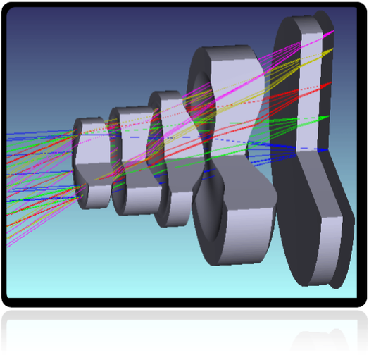
Refer to the figure on right side, representing a multiplet with six optic elements in a smartphone. Feynman’s point of view about the sum over histories encounters here an immediate application when trying to imagine the total of all of the superpositions involved in the formation of what we name image. Their number is mind boggling yet when trying to simplify the evaluation imagining each one lens of infinitesimal thickness, so to abstract by the diffraction and refraction effects between consecutive atoms in a lens. Their total grows further starting to consider that the majority of atoms, have plenty of substructures (e.g., quarks) which can mutually interfere. We are trying to clear that when Nature is closely and thoroughly observed, it shows those numbers with hundredths of zeros which appear in others of these web pages.
![]() 6-lenses optic multiplet in a common smartphone, illustrates superposition's complexity
6-lenses optic multiplet in a common smartphone, illustrates superposition's complexity
Pages on related subjects:


Other subjects:


- Fill level inspection tech: a TCO point of view
- Physics of Triggering
- What Detectors detect ?
- Electromagnetic Measurements of Food, Beverages and Pharma: an Information Retrieval problem
- Binary Classification fundamentals
- Electronic Inspectors’ nonclassic components
- Measures in a Decohering Environment
- FIFO: Bottling Quality Control applications of an idea born to manage the highest production performances
- Photodetectors fundamental definitions
- Media download
- Containers